43 pivot table excel row labels side by side

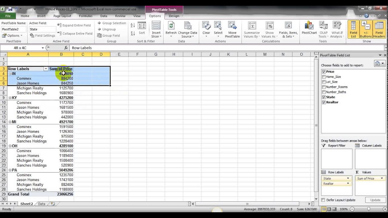
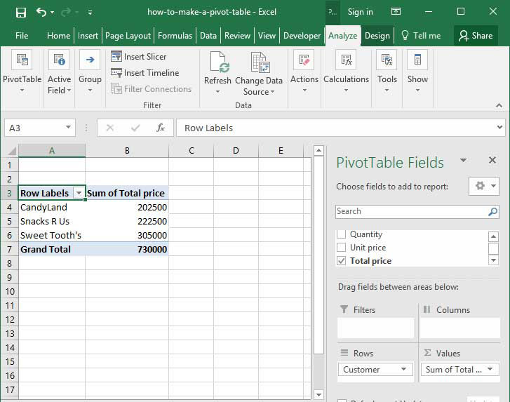
Pivot table row labels in separate columns • AuditExcel.co.za Our preference is rather that the pivot tables are shown in tabular form (all columns separated and next to each other). You can do this by changing the report format. So when you click in the Pivot Table and click on the DESIGN tab one of the options is the Report Layout. Click on this and change it to Tabular form. blog.hubspot.com › marketing › how-to-create-pivotHow to Create a Pivot Table in Excel: A Step-by-Step Tutorial Dec 31, 2021 · After you've completed Step 3, Excel will create a blank pivot table for you. Your next step is to drag and drop a field — labeled according to the names of the columns in your spreadsheet — into the Row Labels area. This will determine what unique identifier — blog post title, product name, and so on — the pivot table will organize ...

How to Customize Your Excel Pivot Chart Data Labels - dummies The Data Labels command on the Design tab's Add Chart Element menu in Excel allows you to label data markers with values from your pivot table. When you click the command button, Excel displays a menu with commands corresponding to locations for the data labels: None, Center, Left, Right, Above, and Below. None signifies that no data labels ...

Pivot table excel row labels side by side

PivotTable Columns Side by Side - Microsoft Community Within that division 2 for Nebraska and 3 for Caufield. I want represent that data in the pivottable with the Division and Branch side by side in columns, like this: Division Branch Branch Count Constance Total 5 Nebraska 2 Caufieled 3 Horace Total 6 Clancy 4 Harken 2 Grand Total 11 It doesn't have to be exactly like this. en.wikipedia.org › wiki › Pivot_tablePivot table - Wikipedia Pivot tables are not created automatically. For example, in Microsoft Excel one must first select the entire data in the original table and then go to the Insert tab and select "Pivot Table" (or "Pivot Chart"). The user then has the option of either inserting the pivot table into an existing sheet or creating a new sheet to house the pivot table. How to Use Excel Pivot Table Label Filters Watch the steps in this short video, and the written instructions are below the video. Play. To change the Pivot Table option to allow multiple filters: Right-click a cell in the pivot table, and click PivotTable Options. Click the Totals & Filters tab Under Filters, add a check mark to 'Allow multiple filters per field.'.

Pivot table excel row labels side by side. powerspreadsheets.com › excel-pivot-table-groupExcel Pivot Table Group: Step-By-Step Tutorial To Group Or ... In fact, as mentioned in Excel 2016 Pivot Table Data Crunching: Each time you create a new pivot table in Excel 2016, Excel automatically shares the pivot cache. Pivot Cache sharing has several benefits. Most notably, as I mention above, it reduces memory requirements and file size vs. the scenario where the Pivot Cache isn't shared. Multi-level Pivot Table in Excel (In Easy Steps) First, insert a pivot table. Next, drag the following fields to the different areas. 1. Order ID to the Rows area. 2. Amount field to the Values area. 3. Country field and Product field to the Filters area. 4. Next, select United Kingdom from the first filter drop-down and Broccoli from the second filter drop-down. Pivot Table Row Labels In the Same Line - Beat Excel! First make a pivot table with required fields. Arrange the fields as shown in left picture. Your initial table will look like right picture. Now click on "Error Code" and access field settings. First check "None" option in "Subtotals & Filters" tab to disable totals after every row. How to make row labels on same line in pivot table? Make row labels on same line with PivotTable Options You can also go to the PivotTable Options dialog box to set an option to finish this operation. 1. Click any one cell in the pivot table, and right click to choose PivotTable Options, see screenshot: 2.

Excel tutorial: How to filter a pivot table by rows or columns When you add a field as a row or column label in a pivot table, you automatically get the ability to filter the results in the table by items that appear in that field. Let's take a look. This pivot table is displaying just one field: Total Sales. After we add Product as a row label, notice that a drop-down arrow appears in the header area. Pivot table row labels side by side - Excel Tutorials You can copy the following table and paste it into your worksheet as Match Destination Formatting. Now, let's create a pivot table ( Insert >> Tables >> Pivot Table) and check all the values in Pivot Table Fields. Fields should look like this. Right-click inside a pivot table and choose PivotTable Options…. Check data as shown on the image below. How to Flatten and repeat Row Labels in a Pivot Table Excelerator BI 4.5K subscribers Subscribe This video shows you how to easily flatten out a Pivot Table and make the row labels repeat. This is useful if you need to export your data and share it... › excelpivottablesetupHow to Set Up Excel Pivot Table for Beginners Apr 19, 2022 · That will make it easier for Excel to build the pivot table. Then, click the Insert tab on the Excel Ribbon. There are two pivot table commands on the Insert tab of the Excel Ribbon, and both options are explained below. Recommended PivotTables - select a layout and Excel creates a quick pivot table; PivotTable - Excel creates a blank pivot table

Pivot Table Multiple Row Labels? [SOLVED] - Excel Help Forum Is it possible to have two Row Labels showing in a Pivot Table, instead of one showing as a sub-category of the other. I have a spreadsheet that shows the status (Design, Development, Testing, Live), owner and engineer for software. I currently have to have two separate pivot tables: 1) showing count of software in each status for each owner. Pivot Table column label from horizontal to vertical Pivot Table column label from horizontal to vertical After pivot table and with grouping, some column labels have been showed but the caption is on the top. What i want is put the column header at the left of the row as vertical red text show as below. However, i cannot do this, it said "We cant change this part of pivot table". Design the layout and format of a PivotTable In the PivotTable, right-click the row or column label or the item in a label, point to Move, and then use one of the commands on the Move menu to move the item to another location. Select the row or column label item that you want to move, and then point to the bottom border of the cell. Excel Pivot Table Report - Sort Data in Row & Column Labels & in Values ... The dialog box can be launched in many ways: under the 'PivotTable Tools' tab on the ribbon -> click 'Options' tab -> in the 'Sort' group click on 'Sort'; right-click a cell in the values area in the Pivot Table report and from the list of commands which opens, point to 'Sort' and click on 'More Sort Options' in the list.

Pivot table row labels side by side – Excel Tutorials

How do I have multiple row labels in a pivot table? Click any cell in your pivot table, and the PivotTable Tools tab will be displayed. Under the PivotTable Tools tab, click Design > Report Layout > Show in Tabular Form, see screenshot: And now, the row labels in the pivot table have been placed side by side at once, see screenshot:.

Use Excel PivotTables to quickly analyze grades - Extra Credit

07 Pivot Table side by side row labels - groups.google.com - Go to PivotTable Tools, then Options - in the Active Field, select Field Settings - In the Field Settings box, select the 2nd tab 'Layout & Print' - Under 'Show item labels in outline form',...

Pivot table row labels in separate columns • AuditExcel.co.za

How to add side by side rows in excel pivot table - AnswerTabs To display more pivot table rows side by side, you need to turn on the Classic PivotTable layout and modify Field settings. For example will be used the following table: You have to right-click on pivot table and choose the PivotTable options. Then swich to Display tab and turn on Classic PivotTable layout:

Multiple Row Filters in Pivot Tables - YouTube

› pivot-table-tips-and-tricks101 Advanced Pivot Table Tips And Tricks You Need To Know Apr 25, 2022 · As a new pivot table user I LOVE this website – very well written! I do have a unique issue I’m hoping to get assistance with. I have a pivot table built out with multiple rows and columns pertaining to new hire information. My boss likes the option to “drill down” and view the source data.

Create a Pivot Table in Excel - The Complete Beginners Guide - QuickExcel

› excel-pivot-taHow to Create Excel Pivot Table [Includes practice file] Jan 15, 2022 · How to Create Excel Pivot Table. There are several ways to build a pivot table. Excel has logic that knows the field type and will try to place it in the correct row or column if you check the box. For example, numeric data such as Precinct counts tend to appear to the right in columns. Textual data, such as Party, would appear in rows.

Excel: Select Pivot Table Parts For Formatting - Excel Articles

Automatic Row And Column Pivot Table Labels - How To Excel At Excel Select the data set you want to use for your table The first thing to do is put your cursor somewhere in your data list Select the Insert Tab Hit Pivot Table icon Next select Pivot Table option Select a table or range option Select to put your Table on a New Worksheet or on the current one, for this tutorial select the first option Click Ok

How to reset a custom pivot table row label

How to Add Rows to a Pivot Table: 9 Steps (with Pictures) Click anywhere in your pivot table. This opens the pivot table editor on the right side of Google Sheets. 3. Click Add under "Rows." It's in the left side of the pivot table editor. A list of fields will expand on the menu. 4. Click the name of the field you want to add as a row.

Excel pivot table hides complete row when blank values or labels are filtered - Super User

How to make row labels on same line in pivot table in excel #ExcelMaster, #PivotTable, #ExcelHow to make row labels on same line in pivot table in excelHow to show multiple rows in pivot table in excel

Pivot Table in Microsoft Excel - Pivot Table Field List Report Functions of Filter Column Labels ...

How to repeat row labels for group in pivot table? - ExtendOffice In Excel, when you create a pivot table, the row labels are displayed as a compact layout, all the headings are listed in one column. Sometimes, you need to convert the compact layout to outline form to make the table more clearly. But in tphe outline layout, the headings will be displayed at the top of the group.

How to use a pivot table in Excel 2013 - Quora

Excel Pivot tables 2007 Row labels side by side - MrExcel Message Board Try selecting a cell in the pivot table and then: PivotTable Tools tab Design tab Report Layout button in the Layout group Select "Show in tabular form" Click to expand... Thank you! This was such an easy solution to a really hard to find problem. You must log in or register to reply here. Similar threads R Pivot Table Editor RodneyC Mar 23, 2022

Pivot Table Tip- Assign The Correct Row And Column Labels Quickly - How To Excel At Excel

› createpivottableHow to Create a Pivot Table in Excel Create a Pivot Table in Excel. Follow these easy steps to create an Excel pivot table, so you can quickly summarize Excel data. Watch the short video to see the steps, or follow the written steps. Get the free workbook, to follow along. There's also an interactive pivot table below, that you can try, before you build your own!

Design your Pivot Table in Excel | Excel in Excel

Pivot Table Row Labels • AuditExcel.co.za Right click on the Row Labels again - go to Field Settings. Look at Layout and Print. At the moment it is ticked as "show item labels in tabular form" - if I said please show the items labels in "outline form" and say OK you will see how the Pivot Table looks changes. Go back to Layout and Print and say "please display labels from ...

Excel Master Series Blog: Simplifying Excel Pivot Table and Pivot Chart Setup

Hide Excel Pivot Table Buttons and Labels Hide Excel Pivot Table Buttons. If you leave those pivot table buttons showing, it's easy for people to change the filters that you applied, or to hide the region names (accidentally, or on purpose!). To discourage people from changing the pivot table layout, follow these steps to make a couple of changes to the display settings.

Pivot Table Row Labels Side By Side | Decorations I Can Make

multiple fields as row labels on the same level in pivot table Excel ... multiple fields as row labels on the same level in pivot table Excel 2016 I am using Excel 2016. I have data that lists product models along with relevant data and also production volumes by month. Part of the relevant data are about 5 common part columns with the part # that applies to each model under the appropriate column.

Pivot Table Multiple Row Labels Side By Side | Decorations I Can Make

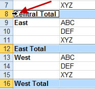
Repeat item labels in a PivotTable - support.microsoft.com Right-click the row or column label you want to repeat, and click Field Settings. Click the Layout & Print tab, and check the Repeat item labels box. Make sure Show item labels in tabular form is selected. Notes: When you edit any of the repeated labels, the changes you make are applied to all other cells with the same label.

Share :